NBHF Clusters: Streamlined Results

Intro

We want to identify clusters within our training set before we make our classifier learn from it. There are two objectives for unsupervised clustering:

1. Look across species to identify whether species classes form separate clusters (Section 1).
   • The existence of clusters suggests that there are meaningful differences between classes that the classifier can be trained to recognize.
2. Look within species classes to assess variability among events (Section 2).
   • The existence of clusters within an individual species class may indicate that there are outlying events with anomalous features that should be excluded from the training set.

Objective 1

Method

set.seed(123)

# slice sample of 200 clicks from each species
samp <- train.ec %>%
  group_by(species) %>%
  slice_sample(n=120) %>%
  ungroup()

samp_rm <- samp %>% 
  # drop metadata
  select(-c(UID:noiseLevel, BinaryFile, eventLabel,detectorName, db)) %>% 
  # drop variables to avoid creating artifacts in the cluster plot.
  select(species, eventId, duration:peak, Q_10dB:centerkHz_3dB) %>%
  # perform logarithmic transform for non-normally distributed variables
  mutate(log_duration = log(duration), log_Q_3dB = log(Q_3dB), log_Q_10dB = log(Q_10dB), .keep = "unused")

# calculate Euclidean distances
dist <- samp_rm %>%
  select(-c(species, eventId)) %>%
  mutate(id = 1:n()) %>%
  column_to_rownames("id") %>%
  scale() %>%
  dist(method="euclidean")

cl <- densityClust(dist)
# set rho and delta values
cl <- findClusters(cl, rho=10, delta=2.5)

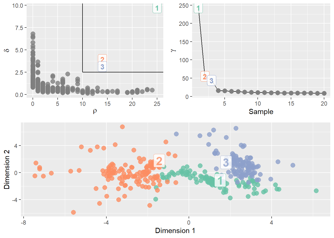
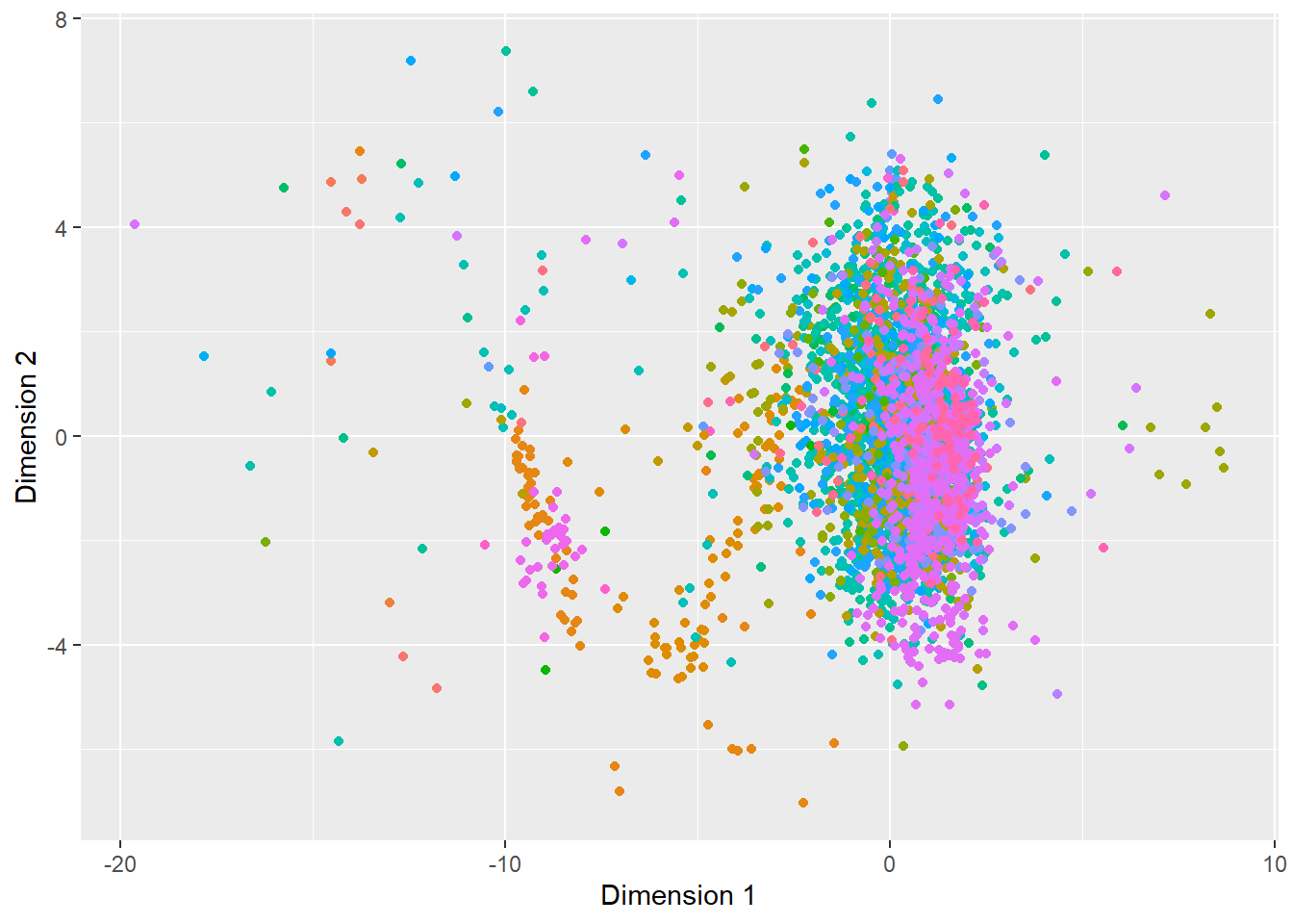
Using the above method, the density clustering algorithm formed the clusters shown in Figure 1. The counts of each species in each of the resulting clusters is given in Table 1. The MDS plot is shown with the points colored by species in Figure 2.

Figure 1: Density clusters with Four clusters formed with ρ=25 and δ=2

Table 1: Table of cluster assignments

    
       1   2   3
  ks   6 111   3
  pd  86  22  12
  pp  18   6  96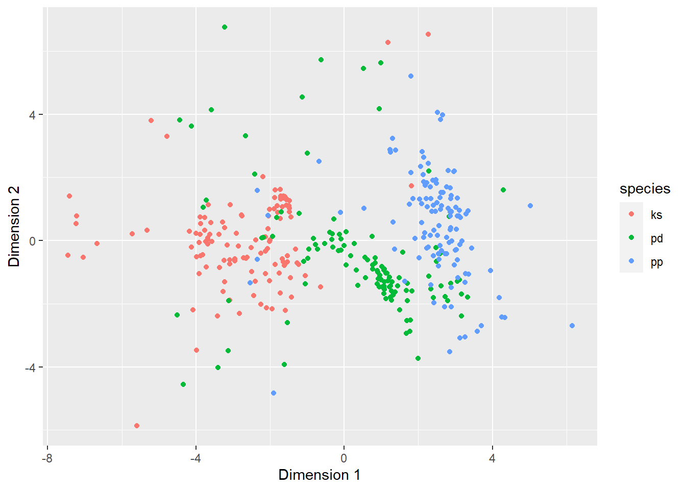

Figure 2: MDS plot showing distances between clicks in the training set, colored by species

Discussion

• Each of the three clusters appears to be dominated by a different species class:
  • Cluster 1: Dall’s porpoise
  • Cluster 2: Kogia
  • Cluster 3: harbor porpoise
• The MDS plot similarly shows that clicks separate into three different clusters by species class.

Objective 2

We will now subset the training data by species and then re perform density clustering to identify anomalous events.

Method

set.seed(123)

samp_rm <- train.ec %>% 
  # drop metadata
  select(-c(UID:noiseLevel, BinaryFile, eventLabel,detectorName, db)) %>% 
  # drop variables to avoid creating artifacts in the cluster plot.
  select(species, eventId, duration:peak, Q_10dB:centerkHz_3dB) %>%
  # perform logarithmic transform for non-normally distributed variables
  mutate(log_duration = log(duration), log_Q_3dB = log(Q_3dB), log_Q_10dB = log(Q_10dB), .keep = "unused")


sp <- c("ks", "pd", "pp")
# subset data by species
samp_sp <- lapply(sp, \(x) filter(samp_rm, species==x))
# create distance matrices.
dist_sp <- lapply(samp_sp, \(s) s %>% select(-c(species, eventId)) %>% mutate(id = 1:n()) %>% column_to_rownames("id") %>% scale() %>% dist())
cl_sp <- lapply(dist_sp, densityClust)
# Perform density clustering. Static values chosen for rho and delta.
# This decision does not seem to be critical, because the algorithm strongly favors a single cluster for each species.
cl_sp <- lapply(cl_sp, findClusters, delta = 8, rho = 5)

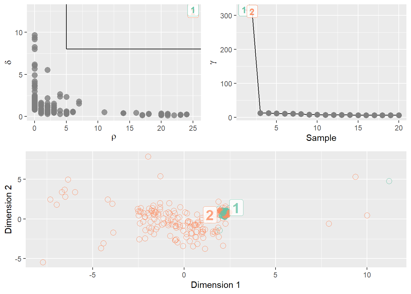
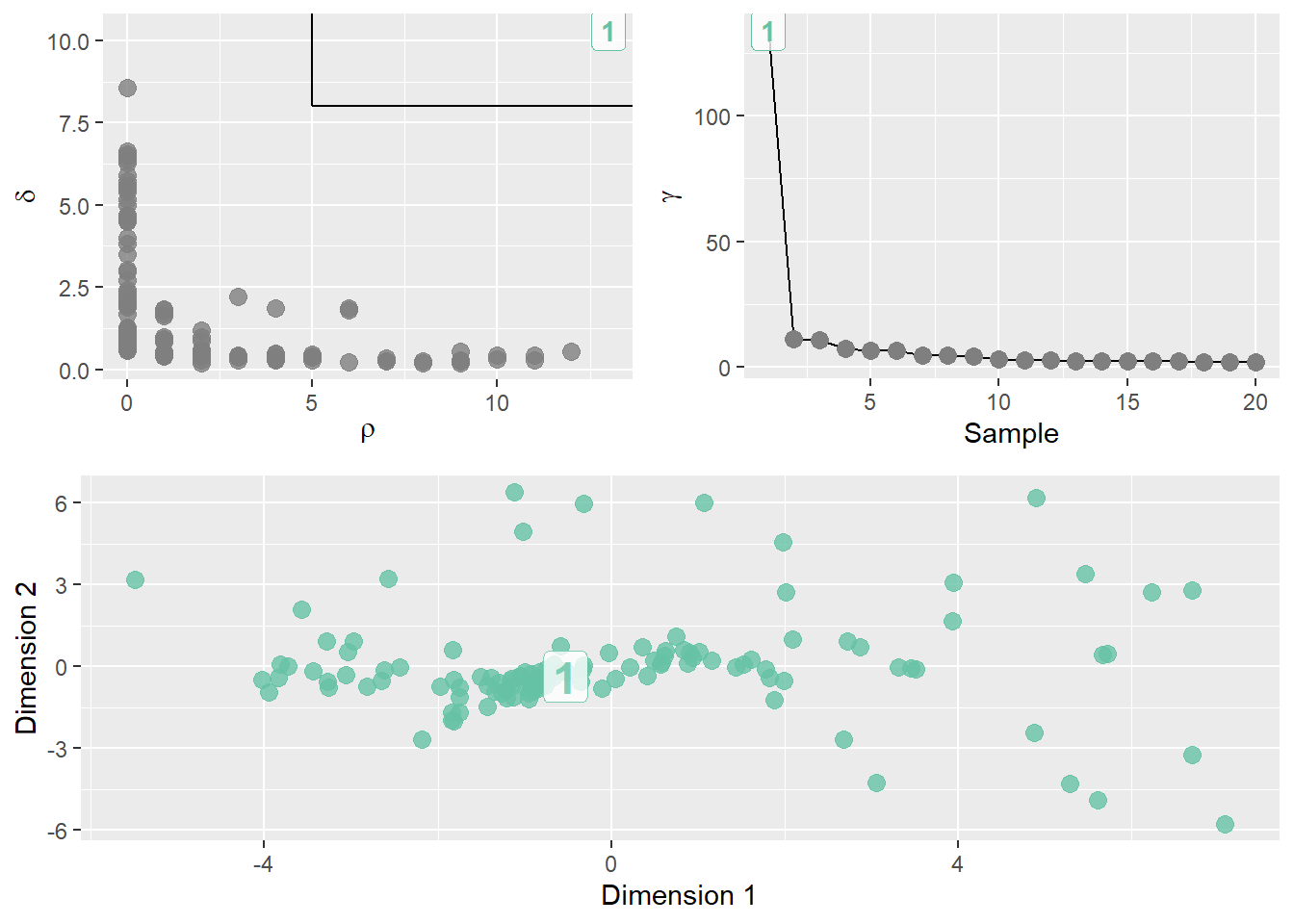
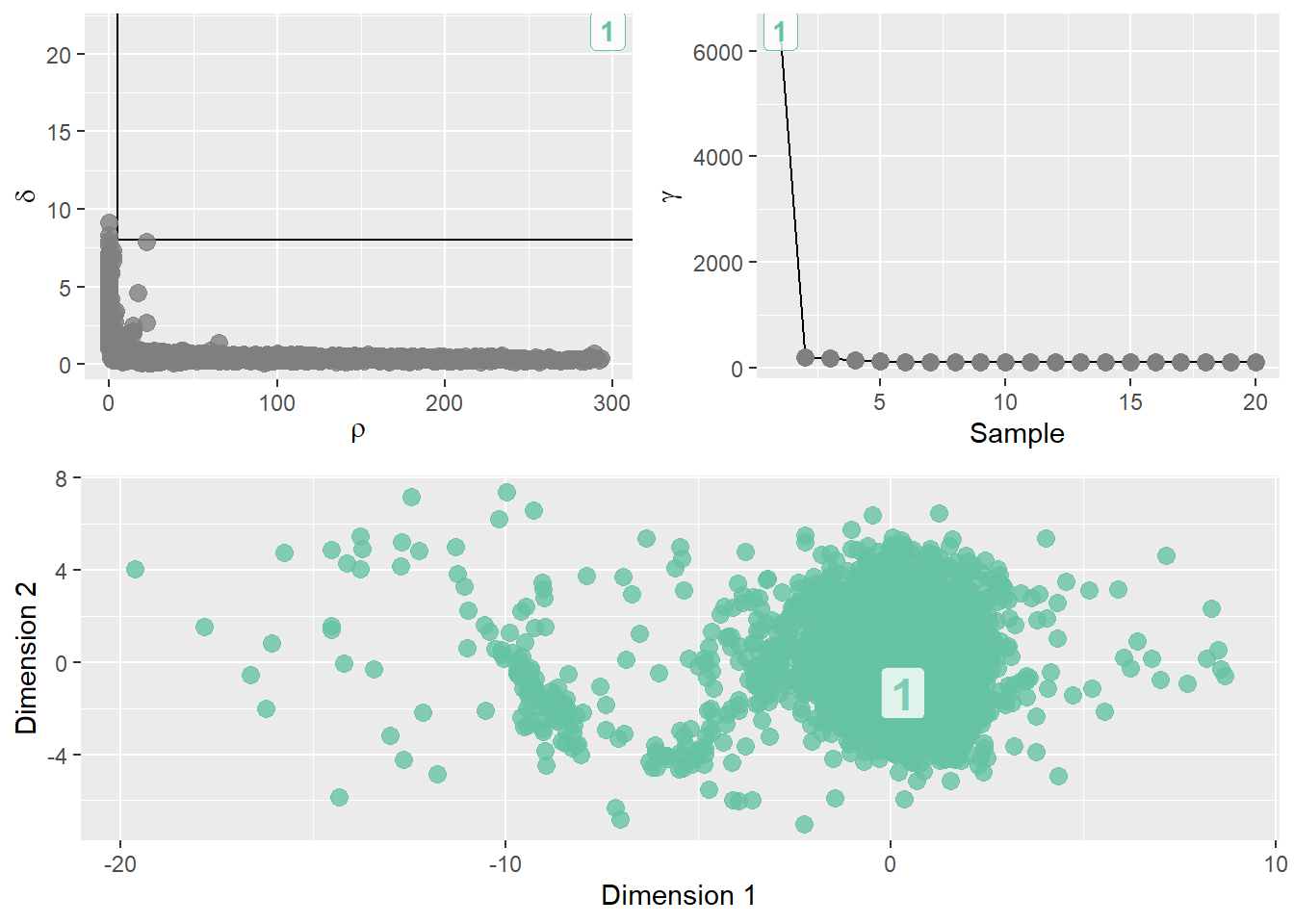
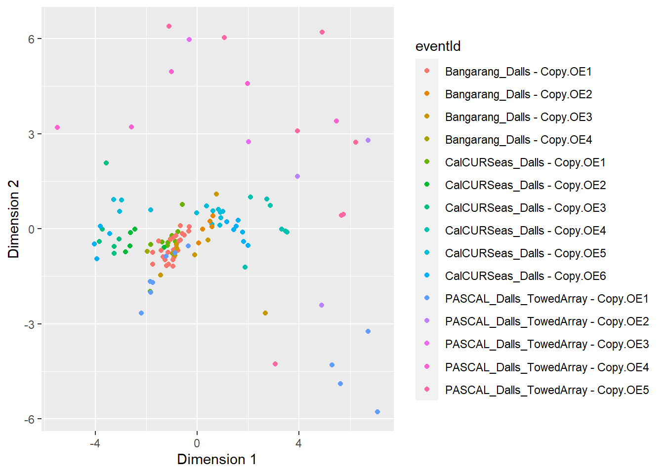
Figure 3 shows the resulting density cluster plots and Figure 4 shows the plots with the points colored by event.

(a) Kogia

(b) Dall’s porpoise

(c) Harbor porpoise

Figure 3: Click clusters for each species class

Warning: The `<scale>` argument of `guides()` cannot be `FALSE`. Use "none" instead as
of ggplot2 3.3.4.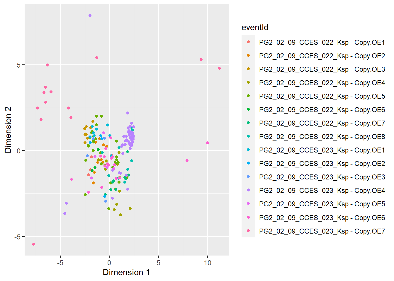

(a) Kogia

(b) Dall’s porpoise

(c) Harbor porpoise

Figure 4: MDS plot showing distances between clicks, colored by event. Legend is hidden for harbor porpoise due to large number of events.

Discussion

• The density clustering algorithm appears to strongly favor a single cluster for both Dall’s porpoise and harbor porpoise, suggesting that there are no outlying events.
• When points are colored by event, variation among events is more evident. This variation does not appear to be strong enough to manifest as more than one density-based cluster, except in the case of Kogia.
• In the case of Kogia, a solution of two clusters appears to be favored.
  • Cluster 1, the smaller cluster, derives most of its clicks from the event identified as PG2_02_09_CCES_023_Ksp - Copy.OE4.
  • This same event, which happens to be the largest Kogia event in the training set, has the majority of its clicks in the dominant cluster, cluster 2. This is shown in Table 2.
  • In the Kogia distance plot, you can see a tight cluster of purple dots corresponding to the event in question. This appears to be the signal that is causing the density clustering algorithm to create a second cluster.

Table 2: Cluster assignments of Kogia clicks, separated by event

                                   
                                     1  2
  PG2_02_09_CCES_022_Ksp - Copy.OE1  0  4
  PG2_02_09_CCES_022_Ksp - Copy.OE2  0  9
  PG2_02_09_CCES_022_Ksp - Copy.OE3  0  9
  PG2_02_09_CCES_022_Ksp - Copy.OE4  0 13
  PG2_02_09_CCES_022_Ksp - Copy.OE5  0 30
  PG2_02_09_CCES_022_Ksp - Copy.OE6  0  3
  PG2_02_09_CCES_022_Ksp - Copy.OE7  1  8
  PG2_02_09_CCES_022_Ksp - Copy.OE8  0 10
  PG2_02_09_CCES_023_Ksp - Copy.OE1  0  7
  PG2_02_09_CCES_023_Ksp - Copy.OE2  0  5
  PG2_02_09_CCES_023_Ksp - Copy.OE3  0  4
  PG2_02_09_CCES_023_Ksp - Copy.OE4 14 38
  PG2_02_09_CCES_023_Ksp - Copy.OE5  0  5
  PG2_02_09_CCES_023_Ksp - Copy.OE6  0 17
  PG2_02_09_CCES_023_Ksp - Copy.OE7  1 12